ML tasks reviews
- Node-level prediction → Node features
- Link-level prediction → Link features
- Graph-level prediction → Graph features

Node-level prediction
$G = (V, E)$가 주어질 때, 함수 $f: V \to \mathbb{R}$를 학습한다.
Goal: 네트워크의 노드의 구조와 위치를 특성화한다.
Node Features
- Node degree
- Node centrality
- Clustering coefficient
- Graphlets
Node Centrality
node degree는 importance를 포착하지 않는다.
node centrality $c_v$는 node importance를 지닌다.
node centrality는 여러 방법이 존재한다
- Eigenvector centrality
- Betweenness centrality
- Closeness centrality
- Others
Node Centrality (1) - Eigenvector Centrality
node $v$의 이웃노드집합을 $N(v)$라 표기하자. 이 때 노드 $v$의 node centrality는 이웃 노드의 centrality의 합계로 정의하면
$$c_v = \cfrac{1}{\lambda}\displaystyle\sum_{u \in N(v)}c_u$$
$\lambda$는 정규화된 상수이다. (아래에 이 값은 인접행렬 $A$의 가장 큰 고윳값임을 보일 것이다.)
그런데 이 정의는 recursive하게 서술되어있다. (centrality를 정의하기 위해 centrality를 이용한다)
위의 서술을 행렬 형태로 서술하면
$$\lambda \mathbf{c} = \mathbf{Ac}$$
즉 centrality $c$는 $A$의 eigenvector임을 알 수 있다.
Node Centrality (2) - Betweenness Centrality
$s$와 $t$의 shortest path에 $v$가 포함되어있으면, 그 노드($v$)는 중요하다고 생각한다.


Node Centrality (3) - Closeness Centrality
$v$가 다른 모든 노드 $u \neq v$에 도달하는 shortest path의 합이 작으면 중요도가 크다고 생각한다.


$A$에서 다른 모든 노드들에 도달하는 최단거리의 길이는 각각 2, 1, 2, 3이므로 $c_A = 1/8$
$D$에서 다른 모든 노드들에 도달하는 최단거리의 길이는 각각 2, 1, 1, 1이므로 $c_D = 1/5$
Clustering Coefficient
$v$의 이웃 노드들이 어떻게 연결되었는지 계산
$$e_v = \cfrac{\text{#(edges among neighboring nodes)}}{\binom{k_v}{2}} \in \left[ 0, 1 \right]$$

Graphlets
Graphlet: Rooted connected induced non-isomorphic subgraph
- induced subgraph: is another graph, formed from a subset of vertices and all of the edges connecting the vertices in the subset.
- graph isomorphism: 동형 그래프
5개의 노드는 73개의 graphet이 존재한다.
Graphlet Degree Vector (GDV): 주어진 노드를 루트로 갖는 graphlet의 개수를 구하는 벡터

Link-level Prediction
- Links missing at random: link 몇개를 제거하고 제거된 link를 predict하도록 한다.
- Links over time: $\left[ t_0, t_0' \right] 에서 정의된 edge가 \left[ t_1, t_1' \right]$ 에서 새로 생기는(혹은 없어지는) edge를 예측
노드 쌍 $(x, y)$에 대하여 점수 $c(x, y)$를 계산하고, 내림차순으로 점수를 정렬한다. 그리고 가장 높은 $n$개의 링크를 예측한다.
Distance-Based Features
Shortest-path distance between two nodes
하지만 이 방법은 이웃의 degree를 capture하지 못하는 문제가 있다.
Local Neighborhood Overlap
두 노드 $v_1, v_2$가 공유하는 이웃노드의 개수로 정의;
- Common neighbors: $\left| N(v_1) \cap N(v_2) \right|$
- Jaccard's coefficient: $\cfrac{\left| N(v_1) \cap N(v_2) \right|}{\left| N(v_1) \cup N(v_2) \right|}$
- Adamic-Adar index: $\displaystyle\sum_{u \in N(v_1) \cap N(v_2)} \cfrac{1}{\log{(k_u)}}$

이 그래프에서 노드 $A, B$의 local neighborhood overlap score를 구하면
$N(A) = \{ C \}$, $N(B) = \{ C, D \}$이므로
- Common neighbors: 1
- Jaccard's coefficient: 1/2 = 0.5
- Adamic-Adar index: \cfrac{1}{\log{4}}
Global Neighborhood Overlap
하지만 local neighborhood feature도 $\left| N(v_1) \cap N(v_2) \right| = \varnothing$이 될 수 있는 문제점이 있다. 그러나 이 경우에도 두 노드가 연결될 가능성은 존재한다.
katz index: 두 노드 쌍의 모든 길이의 walk의 개수. 그래프 인접행렬의 거듭제곱으로 구할 수 있다.
$$P_{uv}^{(K)} = \text{#walks of legth }K \text{ between }u \text{ and }v$$
그리고 $P^{K} = A^K$이므로 (증명 생략) katz index($S$)를 수식으로 전개하면
$$S_{v_1v_2} = \displaystyle\sum_{l=1}^{\infty} \beta^{l} A_{v_1v_2}^{l}$$
$$ \mathbf{S} = \displaystyle\sum_{i=1}^{\infty} \beta^i \mathbf{A}^i = (\mathbf{I} - \beta \mathbf{A})^{-1} - \mathbf{I} $$
이때 $\beta$는 discount factor로 $0 < \beta < 1$이다.
Graph-Level Features
Kernel Method
전통적인 graph-level prediction에서 ML에서 자주 사용된 방법이다.
아이디어: kernel은 feature vector를 대체할 수 있다.
Quick introduction to Kernels
$K(G, G') \in \mathbb{R}$
Kernel matrix $\mathbf{K} = \left( K(G, G') \right)_{G, G'}$은 반드시 양의 semidefinite여야 한다.(예. 양의 교윳값)
$K(G, G') = \phi(G)^T \phi(G')$를 만족하는 feature representation $\phi \left( \cdot \right)$가 존재한다.
Graph Kernels: 두 그래프의 유사성을 측정하는 핵
- Graphlet Kernel → 계산산의 이유로 잘 사용하지 않음
- Weisfeiler-Lehman Kernel → 계산상의 효율성 + GNN과 밀접한 연관성
- Others: Random-walk kernel, Shortest-path graph kernel, etc
1)과 2) 모두 Bag-of-* 의 아이디어로 커널을 구성한다. (bag-of-node count, bag-of-degree of node로 커널을 구성하면 서로 다른 두 그래프가 같은 그래프로 취급되는 문제점이 있다.)
Graphlet Kernel
Key idea: graphlet의 개수를 세는 커널
graphlet list $g_k = (g_1, g_2, \dots , g_{n_k})$에 대하여 graphlet count vector $\mathbf{f}_G \in \mathbb{R}^{n_k}$는 다음과 같이 정의된다
$$(\mathbf{f}_G)_i = \text{#}(g_i \subseteq G) \text{ for } i=1, 2, \dots , n_k$$

따라서 graphlet kernel은 두 그래프의 크기가 다른 경우도 고려하여(feature vector를 정규화하여) 다음과 같이 계산할 수 있다.
$$L(G, G') = \mathbf{h}_G^T \mathbf{h}_{G'} \text{ where } \mathbf{h}_G = \cfrac{\mathbf{f}_G}{Sum(\mathbf{f}_G)}$$
그러나 시간복잡도가 $O(nd^{k-1})$이고 subgraph의 isomorphism test는 NP-hard로 알려져있기 때문에 계산효율성이 매우 떨어진다.
Weisfeiler-Lehman Kernel (WL-kernel)
바이스파일러-리만 알고리즘을 이용한다.
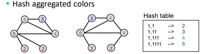
노드집합 $V$를 갖는 그래프 $G$가 있을 때, 각 노드 $v$마다 초기 색상 $c^{(0)}(v)$를 할당한다.
그리고 $K$번 반복적으로 노드의 색을 refine한다
$$c^{(k+1)}(v) = \text{HASH} \left( \left\{ c^{(k)}(v), \left\{ c^{(k)}(u) \right\}_{u \in N(v)} \right\} \right)$$
$\text{HASH}$는 다른 입력에 대하여 다른 색을 매핑하는 함수이다.
아래 예시를 통해 WL-kernel을 계산하는 방법을 보자
| Color Refinement 예시 |
 |
 |
 |
 |
 |
 |
 |
WL kernel은 계산이 효율적이다. (#edges 에 선형 비례한다)
'스터디 > 인공지능, 딥러닝, 머신러닝' 카테고리의 다른 글
| [CS224w] 5. A General Perspective on GNNs (2), 아키텍처 (0) | 2023.03.10 |
|---|---|
| [CS224w] 4. Graph Neural Networks (0) | 2023.03.07 |
| [CS224w] Colab 1 - Node Embeddings (1) | 2023.03.06 |
| [CS224W] 3. Node Embeddings (0) | 2023.01.28 |
| [CS224W] 1. Introduction (0) | 2023.01.23 |


