강의자료 1~3 기반 colab 프로그래밍 과제이다.
- 1. Introduction
- 2. Feature Engineering for Machine Learning in Graphs
- 3. Node Embeddings
Dataset
Zachary's karate(가라테) club network라는 그래프 데이터를 이용할 것이다. NetworkX에 내장되어있으니 간단히 불러온다.
import networkx as nx

G = nx.karate_club_graph()
print(type(G))           # <class 'networkx.classes.graph.Graph'>
print(G.is_directed())   # False
그래프를 그려볼 수 있다. 실행할 때마다 그래프 그림이 달라지지만, 당연히 같은 그래프이다.
nx.draw(G, with_labels=True)
Question 1. Average degree of network
이 그래프는 무방향 그래프이므로, 강의자료1의 (무방향 그래프에 대한) node degree 정의를 살펴보면
\[ \bar{k} = \cfrac{2E}{N} \]
따라서 함수의 파라미터로 들어온 $E, N$을 이용한다.
def average_degree(num_edges, num_nodes):
  # TODO: Implement this function that takes number of edges
  # and number of nodes, and returns the average node degree of
  # the graph. Round the result to nearest integer (for example
  # 3.3 will be rounded to 3 and 3.7 will be rounded to 4)

  avg_degree = 0

  ############# Your code here ############
  avg_degree = round(2 * num_edges/ num_nodes)
  #########################################

  return avg_degree

num_edges = G.number_of_edges()
num_nodes = G.number_of_nodes()
avg_degree = average_degree(num_edges, num_nodes)
print("Average degree of karate club network is {}".format(avg_degree))

----- result -----
Average degree of karate club network is 0
Question 2. Average clustering coefficient of network
강의자료2에서는, 노드 $v$가 이웃 노드들과 얼마나 연결되어있는지 측정하는 지표가 clustering coefficient이다.
\[ e_v = \cfrac{\text{# edges among neighboring nodes}}{\dbinom{k_v}{2}} \in [0, 1] \]
위키피디아의 정의는
\[ C_i = \cfrac{1}{k_i(k_i - 1)} \sum_{j, k}A_{ij}A_{jk}A_{ki} \ \mathrm{where} \ A \mathrm{\ is \ adjacency\ matrix} \]
따라서 average clustering coefficient는 NetworkX 공식문서에 따르면
\[ C = \cfrac{1}{n}\sum_{v \in G}c_v \ \mathrm{where} \ n \text{ is a number of nodes in } G \]
NetworkX 자체 모듈로 average_clustering을 구할 수 있다.
def average_clustering_coefficient(G):
  # TODO: Implement this function that takes a nx.Graph
  # and returns the average clustering coefficient. Round
  # the result to 2 decimal places (for example 3.333 will
  # be rounded to 3.33 and 3.7571 will be rounded to 3.76)

  avg_cluster_coef = 0

  ############# Your code here ############
  ## Note:
  ## 1: Please use the appropriate NetworkX clustering function
  avg_cluster_coef = nx.average_clustering(G)
  avg_cluster_coef = round(avg_cluster_coef, 2)
  #########################################

  return avg_cluster_coef

avg_cluster_coef = average_clustering_coefficient(G)
print("Average clustering coefficient of karate club network is {}".format(avg_cluster_coef))

# Average clustering coefficient of karate club network is 0.57
Question 3. PageRank of network
(웹 페이지 기반 그래프에서) PageRank는 그래프에서 노드의 중요도를 평가하는 지표 중에 하나다. $i$번째 페이지(노드)의 중요도를 $r_i$, 링크의 개수를 $d_i$라 할 때(degree라 해도 무방하다) 각 링크는 $r_i / d_i$의 vote를 얻는다. 이때 $j$번째 페이지의 중요도 $r_j$는
\[ r_j = \sum_{i \to j}\cfrac{r_i}{d_i} \]
라고 한다.
PageRank 알고리즘은 랜덤 검색자가 링크를 통해 특정 페이지에 도달할 확률 분포다. 랜덤으로 페이지에 도달할 확률을 $\beta$라 하면
$$r_j = \sum_{i \rightarrow j} \beta \frac{r_i}{d_i} + (1 - \beta) \frac{1}{N}$$
def one_iter_pagerank(G, beta, r0, node_id):
  # TODO: Implement this function that takes a nx.Graph, beta, r0 and node id.
  # The return value r1 is one interation PageRank value for the input node.
  # Please round r1 to 2 decimal places.

  r1 = 0

  ############# Your code here ############
  ## Note:
  ## 1: You should not use nx.pagerank
  for node in G.neighbors(node_id):
    r1 += beta * r0 / G.degree[node]
  r1 += (1 - beta) / G.number_of_nodes()
  #########################################

  return r1

beta = 0.8
r0 = 1 / G.number_of_nodes()
node = 0
r1 = one_iter_pagerank(G, beta, r0, node)
print("The PageRank value for node 0 after one iteration is {}".format(r1))

# The PageRank value for node 0 after one iteration is 0.12810457516339868
Question 4. (raw) Closeness centrality of network
closeness centrality는 $c(v) = \frac{1}{\sum_{u \neq v}\text{shortest path length between } u \text{ and } v}$ 로 정의된다.
NetworkX는 closeness centrality를 계산해주는 모듈이 있는데, 이는 위의 정의와 다르게 정규화되어있다.
\[ C(u) = \cfrac{n-1}{\sum_{v=1}^{n-1}d(v, u)}, \text{where } d(v, u) \text{ is the shortest-path distance between } u \text{ and } v \]
def closeness_centrality(G, node=5):
  # TODO: Implement the function that calculates closeness centrality
  # for a node in karate club network. G is the input karate club
  # network and node is the node id in the graph. Please round the
  # closeness centrality result to 2 decimal places.

  closeness = 0

  ## Note:
  ## 1: You can use networkx closeness centrality function.
  ## 2: Notice that networkx closeness centrality returns the normalized
  ## closeness directly, which is different from the raw (unnormalized)
  ## one that we learned in the lecture.
  closeness = nx.closeness_centrality(G, u=node)
  n_connected = len(nx.node_connected_component(G, node))
  closeness /= (n_connected - 1)
  closeness = round(closeness, 2)
  #########################################

  return closeness

node = 5
closeness = closeness_centrality(G, node=node)
print("The node 5 has closeness centrality {}".format(closeness))

# The node 5 has closeness centrality 0.01
Question 5. Edge List of graph using PyTorch
def graph_to_edge_list(G):
  # TODO: Implement the function that returns the edge list of
  # an nx.Graph. The returned edge_list should be a list of tuples
  # where each tuple is a tuple representing an edge connected
  # by two nodes.

  edge_list = []

  ############# Your code here ############
  edge_list = list(G.edges)

  #########################################

  return edge_list

def edge_list_to_tensor(edge_list):
  # TODO: Implement the function that transforms the edge_list to
  # tensor. The input edge_list is a list of tuples and the resulting
  # tensor should have the shape [2 x len(edge_list)].

  edge_index = torch.tensor([])

  ############# Your code here ############
  edge_index = torch.tensor(edge_list).T
  #########################################

  return edge_index

pos_edge_list = graph_to_edge_list(G)
pos_edge_index = edge_list_to_tensor(pos_edge_list)
print("The pos_edge_index tensor has shape {}".format(pos_edge_index.shape))
print("The pos_edge_index tensor has sum value {}".format(torch.sum(pos_edge_index)))

# The pos_edge_index tensor has shape torch.Size([2, 78])
# The pos_edge_index tensor has sum value 2535
Question 6. Sample negative edges of network
negative edge는 그래프에 존재하지 않는 edge를 말한다.
주어진 그래프는 양방향 그래프이므로, $(u, v)$가 edge라면 $(v, u)$ 역시 edge임에 유의한다.
import random

def sample_negative_edges(G, num_neg_samples):
  # TODO: Implement the function that returns a list of negative edges.
  # The number of sampled negative edges is num_neg_samples. You do not
  # need to consider the corner case when the number of possible negative edges
  # is less than num_neg_samples. It should be ok as long as your implementation
  # works on the karate club network. In this implementation, self loops should
  # not be considered as either a positive or negative edge. Also, notice that
  # the karate club network is an undirected graph, if (0, 1) is a positive
  # edge, do you think (1, 0) can be a negative one?

  neg_edge_list = []

  ############# Your code here ############
  for i in G.nodes():
    for j in G.nodes():
      if (i, j) in G.edges(): continue
      if (j, i) in G.edges(): continue
      neg_edge_list.append((i, j))
      neg_edge_list.append((j, i))

  neg_edge_list = random.sample(neg_edge_list, num_neg_samples)
  #########################################

  return neg_edge_list

# Sample 78 negative edges
neg_edge_list = sample_negative_edges(G, len(pos_edge_list))

# Transform the negative edge list to tensor
neg_edge_index = edge_list_to_tensor(neg_edge_list)
print("The neg_edge_index tensor has shape {}".format(neg_edge_index.shape))

# Which of following edges can be negative ones?
edge_1 = (7, 1)
edge_2 = (1, 33)
edge_3 = (33, 22)
edge_4 = (0, 4)
edge_5 = (4, 2)

############# Your code here ############
## Note:
## 1: For each of the 5 edges, print whether it can be negative edge
for (u, v) in [edge_1, edge_2, edge_3, edge_4, edge_5]:
  if (u, v) not in pos_edge_list and (v, u) not in pos_edge_list:
    print(f'{(u, v)} is a negative edge of G')
  else:
    print(f'{(u, v)} is not a negative edge of G')
#########################################

The neg_edge_index tensor has shape torch.Size([2, 78])
(7, 1) is not a negative edge of G
(1, 33) is a negative edge of G
(33, 22) is not a negative edge of G
(0, 4) is not a negative edge of G
(4, 2) is a negative edge of G
Question 7. Train the embedding
임베딩 벡터 생성 및 시각화
# Please do not change / reset the random seed
torch.manual_seed(1)

def create_node_emb(num_node=34, embedding_dim=16):
  # TODO: Implement this function that will create the node embedding matrix.
  # A torch.nn.Embedding layer will be returned. You do not need to change
  # the values of num_node and embedding_dim. The weight matrix of returned
  # layer should be initialized under uniform distribution.

  emb = None

  ############# Your code here ############
  emb = nn.Embedding(num_embeddings=num_node, embedding_dim=embedding_dim)
  emb.weight.data = torch.rand(num_node, embedding_dim)
  #########################################

  return emb

emb = create_node_emb()
ids = torch.LongTensor([0, 3])

# Print the embedding layer
print("Embedding: {}".format(emb))

# An example that gets the embeddings for node 0 and 3
print(emb(ids))


def visualize_emb(emb):
  X = emb.weight.data.numpy()
  pca = PCA(n_components=2)
  components = pca.fit_transform(X)
  plt.figure(figsize=(6, 6))
  club1_x = []
  club1_y = []
  club2_x = []
  club2_y = []
  for node in G.nodes(data=True):
    if node[1]['club'] == 'Mr. Hi':
      club1_x.append(components[node[0]][0])
      club1_y.append(components[node[0]][1])
    else:
      club2_x.append(components[node[0]][0])
      club2_y.append(components[node[0]][1])
  plt.scatter(club1_x, club1_y, color="red", label="Mr. Hi")
  plt.scatter(club2_x, club2_y, color="blue", label="Officer")
  plt.legend()
  plt.show()

# Visualize the initial random embeddding
visualize_emb(emb)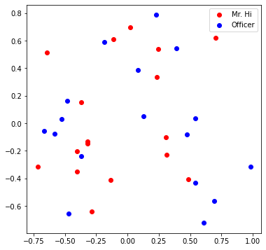
from torch.optim import SGD
import torch.nn as nn

def accuracy(pred, label):
  # TODO: Implement the accuracy function. This function takes the
  # pred tensor (the resulting tensor after sigmoid) and the label
  # tensor (torch.LongTensor). Predicted value greater than 0.5 will
  # be classified as label 1. Else it will be classified as label 0.
  # The returned accuracy should be rounded to 4 decimal places.
  # For example, accuracy 0.82956 will be rounded to 0.8296.

  accu = 0.0

  ############# Your code here ############
  count = torch.sum(torch.round(pred) == label)
  accu = count / pred.shape[0]
  accu = round(accu.item(), 4)
  #########################################

  return accu

def train(emb, loss_fn, sigmoid, train_label, train_edge):
  # TODO: Train the embedding layer here. You can also change epochs and
  # learning rate. In general, you need to implement:
  # (1) Get the embeddings of the nodes in train_edge
  # (2) Dot product the embeddings between each node pair
  # (3) Feed the dot product result into sigmoid
  # (4) Feed the sigmoid output into the loss_fn
  # (5) Print both loss and accuracy of each epoch
  # (6) Update the embeddings using the loss and optimizer
  # (as a sanity check, the loss should decrease during training)

  epochs = 500
  learning_rate = 0.1

  optimizer = SGD(emb.parameters(), lr=learning_rate, momentum=0.9)

  for i in range(epochs):
    ############# Your code here ############
    optimizer.zero_grad()

    z = emb(train_edge) # (1)
    sim = torch.sum(z[0] * z[1], dim=-1) # (2)
    pred = torch.sigmoid(sim) # (3)
    loss = loss_fn(pred, train_label) # (4)
    print(f'Epoch: {i}, Loss: {loss:.4f}, Accuracy: {accuracy(pred, train_label)}') # (5)
    loss.backward() # (6)
    optimizer.step() # (6)
    #########################################

loss_fn = nn.BCELoss()
sigmoid = nn.Sigmoid()

print(pos_edge_index.shape)

# Generate the positive and negative labels
pos_label = torch.ones(pos_edge_index.shape[1], )
neg_label = torch.zeros(neg_edge_index.shape[1], )

# Concat positive and negative labels into one tensor
train_label = torch.cat([pos_label, neg_label], dim=0)

# Concat positive and negative edges into one tensor
# Since the network is very small, we do not split the edges into val/test sets
train_edge = torch.cat([pos_edge_index, neg_edge_index], dim=1)
print(train_edge.shape)

emb = create_node_emb()
train(emb, loss_fn, sigmoid, train_label, train_edge)
임베딩 학습이 끝난 후, 시각화를 해보면, 두 클래스가 잘 분류되어 있는 것(상하로 분리)을 볼 수 있다.
'스터디 > 인공지능, 딥러닝, 머신러닝' 카테고리의 다른 글
| [CS224w] 5. A General Perspective on GNNs (2), 아키텍처 (0) | 2023.03.10 |
|---|---|
| [CS224w] 4. Graph Neural Networks (0) | 2023.03.07 |
| [CS224W] 3. Node Embeddings (0) | 2023.01.28 |
| [CS224W] 2. Feature Engineering for ML in Graphs (0) | 2023.01.23 |
| [CS224W] 1. Introduction (0) | 2023.01.23 |


