Idea of a GNN Layer
벡터들을 하나의 벡터로 압축 + Message와 Aggregation


Message Computation
각 노드들은 메시지를 생성하여 다른 노드들에게 전달하는 직관으로 시작한다.
노드 $u$에서 $l$번째 layer의 메시지 함수 $\mathbf{m}$을 다음과 같이 정의한다.
\[ \mathbf{m}_u^{(l)} = \mathrm{MSG}^{(l)} \left( \mathbf{h}_u^{(l-1)} \right) \]
가장 단순한 예시로 선형 레이어를 생각할 수 있다. $\mathrm{MSG} = \mathbf{W}$
Message Aggregation
각 노드는 이웃 노드들로부터 받은 메시지를 집계할 것이다.
노드 $v$가 메시지를 집계하여 임베딩 $\mathbf{h}_v$를 정의하면
\[ \mathbf{h}_v^{(l)} = \mathrm{AGG}^{(l)} \left( \{ \mathbf{m}_u^{(l)}, u \in N(v) \} \right) \]
$\mathrm{AGG}$의 예시로 $\mathrm{Sum, Mean, Max}$ 등을 사용할 수 있다.
Aggregate를 하면 자기 자신의 노드 $v$의 정보를 잃게 된다. ($\mathbf{h}_v^{l}$이 $\mathbf{h}_v^{(l-1)}$과 전혀 상관없기 때문)
이를 해결하기 위해 $\mathbf{h}$도 같이 계산한다.
개선된 형태는 다음과 같다.
Message는 이웃하는 노드 $N(v)$ 뿐만아니라 자신 $v$의 임베딩 $\mathbf{h}$를 포함하여 메시징을 하고,
Aggregate는 이웃하는 노드의 메시지 뿐만 아니라 자신의 메시지도 포함하여(CONCATor SUM) aggregate한다.
\[ \mathbf{m}_u^{(l)} = \mathrm{MSG}^{(l)} \left( \mathbf{h}_u^{(l-1)} \right), u \in \{ N(v) \cup v \} \]
\[ \mathbf{h}_v^{(l)} = \mathrm{AGG} \left( \{ \mathbf{m}_u^{(l)}, u \in N(v) \}, \mathbf{m}_v^{(l)} \right) \]
추가적으로, message나 aggregation 단계에서 비선형함수(non-linearity activation)을 추가할 수 있다.
Graph Convolution Networks, GCN
GCN의 순서를 바꾸면 Message+Aggregation을 적용한 형태로 바꿀 수 있다.


GraphSAGE

GraphSAGE에서 Message는 $\mathrm{AGG}$이고, Aggregation은 두 단계로 이루어져있다.
GraphSAGE는 AGG에 다양한 함수를 사용한다.
- Mean: $\mathrm{AGG} = \sum_{u \in N(v)} \cfrac{\mathbf{h}_u^{(l-1)}}{|N(v)|}$
- Pool: $\mathrm{AGG} = \mathrm{Mean}\left( \{ \mathrm{MLP}(\mathbf{h}_u^{(l-1)}), \forall_u \in N(v) \} \right)$ Mean 대신에 Max도 사용한다. (symmetric vector function이면 모두 가능)
- LSTM: reshuffled of neighbors에 LSTM을 사용한다. $\mathrm{AGG} = \text{LSTM}([\mathbf{h}_u^{(l-1)}, \forall_u \in \pi \left( N(v) \right) ])$
$l_2$ normalization
GraphSAGE에는 $\mathbf{h}$에 L2 normalization을 적용한다. (Optional) L2 정규화를 하지 않으면 임베딩 벡터들은 각각 다른 scale을 갖는다. (항상 그런 것은 아니지만) 정규화를 하면 성능이 향상되는 효과도 가질 수 있다.
\[ \mathbf{h}_v^{(l)} \leftarrow \cfrac{\mathbf{h}_v^{(l)}}{\Vert \mathbf{h}_v^{(l)} \Vert} \forall_v \in V \]
Graph Attention Networks, GAT
Attention Weights
GCN이나 GraphSAGE에서 $\alpha_{vu} = \cfrac{1}{|N(v)|}$ 였다. $|N(v)|$는 노드의 차수와 동일하므로 모든 노드가 동일한 가중치(weighting factor)를 갖고 있다고 해석할 수 있다.
GAT에서는 모든 모드가 같은 중요도를 가질 것이라고 생각하지 않는다. attention이 중요한 노드를 찾아줄 것이다. 그렇다면 $\alpha_{vu}$ 역시 learnable 해야한다.
Attention Mechanism
노드 $u$가 $v$에게 전달하는 message의 중요도를 $e_{vu}$ (attention coefficient)라 하고 그걸 계산하는 함수를 $a$라 하면
\[ e_{vu} = a \left( \mathbf{w}^{(l)} \mathbf{h}_u^{(l-1)}, \mathbf{w}^{(l)} \mathbf{h}_v^{(l-1)} \right) \]

Normalize $e_{vu}$
$e_{vu}$를 이용하여 final attention weight $\alpha_{vu}$를 계산한다. softmax를 이용하면 $\sum\alpha = 1$이므로 정규화에 이용할 수 있다.
\[ \alpha_{vu} = \cfrac{\text{exp}(e_{vu})}{\sum_{k \in N(v)} \text{exp}(e_{vk})} \]
Weighted sum
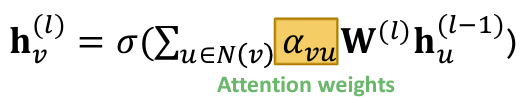
마지막으로 ($v$의 이웃노드들로부터) $v$에 도달하는 모든 가중치를 더해서 임베딩한다.
\[ \mathbf{h}_v^{(l)} = \sigma \left( \sum_{u \in N(v)} \alpha_{vu} \mathbf{W}^{(l)} \mathbf{h}_u^{(l-1)} \right) \]

Note: attention mechanism $a$는 무엇이든 가능하다. 아주 단순한 예로 single-layer neural network 도 가능하다.
e.g. $a = \text{Linear}(\text{Concat}() )$
Multi-head Attention
attention을 더 안정적으로 학습할 수 있다. attention score를 여러개 만들어서 aggregate하는 구조로 만든다.
aggregate는 주로 $\text{CONCAT}$이나 $\text{SUM}$을 이용한다.


Attention mechanism의 장점
- (핵심) 다른 이웃 노드들이 각각 다른 가중치(importance value, $\alpha_{vu}$)를 갖도록 한다.
- 효율적 연산 - 병렬적으로 attentional coefficient를 계산하고, aggregate 역시 병렬적으로 연산이 가능하다.
- 효율적 메모리 사용 - sparse matrix는 최대 $O(V+E)$의 메모리만 사용한다. 고정된 파라미터 수 사용.
- 지역성 - local network neighborhood에만 영향을 받는다. (CNN과 비슷한 성질로 보인다.)
- 귀납적 능력(Inductive capability)
'스터디 > 인공지능, 딥러닝, 머신러닝' 카테고리의 다른 글
| [논문리뷰] TimesNet, Temporal 2D-Variation Modeling for General Time Series Analysis (0) | 2023.04.08 |
|---|---|
| [CS224w] Colab 2 - PyG, OGB, GNN (0) | 2023.03.21 |
| [CS224w] 5. A General Perspective on GNNs (2), 아키텍처 (0) | 2023.03.10 |
| [CS224w] 4. Graph Neural Networks (0) | 2023.03.07 |
| [CS224w] Colab 1 - Node Embeddings (1) | 2023.03.06 |


