
Intuition
아래 2차원 평면에 두 개의 클래스(초록색과 흰색)이 있고, 이를 분류하는 가상의 초평면(2차원이므로 여기서는 직선)을 생각해보자. $B_1$과 $B_2$ 두 직선 모두 두 클래스를 완벽히 구분할 수 있다.
그렇다면 어떤 직선(고차원의 경우 초평면)이 더 좋은 것일까?

직관적으로 우리는 $B_1$이 더 좋은 직선임을 알 수 있다. 그 이유는 각 클래스와의 거리가 가장 멀기 때문이다.

support vector: hyperplane과 가장 가까운 data point
margin: hyperplane과 support vector와의 거리. 일반적으로 margin이 클수록 좋은 SVM이다.
Note: hyperplane은 street로, margin은 street width로 많이 비유된다.
SVM Classifier
아래 예시 데이터(2차원)를 통해 ($n$차원의) SVM의 hyperplane을 구하는 방법으로 확장해보자.

데이터셋 $\mathcal{D}$가 $n$개의 tuple($\mathbf{x}$와 클래스 label인 y의 쌍)로 이루어져있다고 하자. ($n=D = | \mathcal{D}|$) 즉
\[ (\mathbf{x}_1, y_1), \dots, (\mathbf{x}_n, y_n) \]
이때 class label은 $y_i \in \{1, -1 \}$이라 하자.
linearly separable한 hyperplane의 방정식은 $\mathbf{w}^\top \mathbf{x} - b = 0$이라 하자. $\mathbf{w}$는 normal vector, $\mathbf{x}$는 data(input) vector, $b$는 scalar value(bias)이다. (편의상 내적기호 $\cdot$ 대신에 transpose를 이용한 행렬곱으로 표기한다.)
그리고 각 클래스의 경계인 hyperplane 역시 평행하므로 각각 $\mathbf{w}^\top \mathbf{x} - b = 1$, $\mathbf{w}^\top \mathbf{x} - b = -1$ 이라 하자. (위 그림에서 각각 파란색, 초록색 직선을 나타낸다.)
$\mathbf{w}^\top \mathbf{x} - b \ge 1$인 $\mathbf{x}$는 $y=1$인 클래스로, $\mathbf{w}^\top \mathbf{x} - b \le -1$인 $\mathbf{x}$는 $y=-1$로 분류된다.
이를 종합하여 표현하면 다음과 같다.
\[ y_i(\mathbf{w}^\top \mathbf{x} - b) \ge 1, \quad y_i \in \{1, -1 \}, \quad \forall i \in \{1, \dots, n \} \]
그렇다면 우리가 구할 margin의 길이(크기)는 $\cfrac{2}{\Vert \mathbf{w} \Vert}$ 가 되고 이 값이 최대가 되기 위해서는 $\Vert \mathbf{w} \Vert$가 최소가 되어야 한다.
계산의 편의를 위해 $\cfrac{1}{2} \Vert \mathbf{w} \Vert^2$의 최솟값을 찾는 것을 목적함수로 한다.
Primal form
위에서 얻은 식을 정리하면 다음과 같다.
\[ \underset{\mathbf{w}, b}{\text{minimize}} \frac{1}{2} \Vert \mathbf{w} \Vert^2 \]
\[ \text{subject to } y_i(\mathbf{w}^\top \mathbf{x} - b) \ge 1, \quad y_i \in \{1, -1 \}, \quad \forall i \in \{1, \dots, n \} \]
이 함수는 constrained convex quadratic optimization problem이 된다.
Dual form
Lagrangian dual을 이용하여 다음과 같이 표현한다.
$\tilde{L}(\alpha) = \sum_{i=1}^{n} \alpha_i - \cfrac{1}{2}\sum_{i,j} \alpha_i \alpha_j y_i y_j \mathbf{x}_i^\top \mathbf{x}_j$ ($\forall i, j \in \{1, \dots, n \}$)
$\text{subject to } \sum_{i=1}^{n} \alpha_i y_i = 0 \quad (\forall \alpha_i \ge 0)$
Soft Margin
경우에 따라 hyperplane이 모든 데이터를 완벽하게 분류하지 못할 수 있다. 이 경우 soft margin을 도입하여 몇개의 mislabeled sample을 허용하도록 한다.

slack variable $\xi$를 도입하여 degree of misclassification을 측정한다.
\[ \min_{\mathbf{w}, \xi} \biggl\{ \cfrac{1}{2}\Vert \mathbf{w} \Vert^2 + C \sum_{i=1}^{n}\xi_i \biggr\} \]
\[ \text{subject to } y_i(\mathbf{w}^\top \mathbf{x}_i - b) \ge 1 - \xi_i, \quad \xi_i \ge 0, \quad \forall i \in \{1, \dots, n \} \]
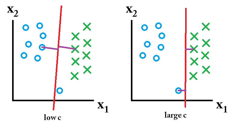
Relationship between $C$ and margin
$C$는 regularization parameter(또는 tuning parameter)이다. ($C > 0$)
$C$의 값이 작으면 regularization이 약화되어 더 많은 misclassification을 더 허용한다. 따라서 margin은 커진다.
$C$의 값이 크면 regularization이 강화되어 misclassification을 더 적게 허용한다. 따라서 margin은 작아진다.
Kernel Trick
When Linearly Inseparable
지금까지 살펴본 SVM은 hyperplane을 구성하는 것이기에 선형의 margin만 가능하다.
그러나 아래의 경우 soft-margin을 이용하여도 선형(혹은 초평면)으로 클래스를 구분할 수 없다.
이 경우, 데이터를 고차원 공간으로 project하여 그곳에서 새로운 hyperplane을 만들어 해결할 수 있다.

Learning in the feature space
training data를 $\Phi$를 이용하여 더 높은 고차원 feature space로 mapping한다.
그리고 feature space에서 margin이 최대가 되는 hyperplane을 구한다.
Input Space
$\text{minimize}_{\alpha} \sum_i \alpha_i - \frac{1}{2}\sum_{i,j}\alpha_i \alpha_j y_i y_j \mathbf{x}_i \mathbf{x}_j$
$\sum_i \alpha_i y_i = 0$
$C \ge \alpha_i \ge 0$
Feature Space
$\text{minimize}_{\alpha} \sum_i \alpha_i - \frac{1}{2}\sum_{i,j}\alpha_i \alpha_j y_i y_j K(\mathbf{x}_i, \mathbf{x}_j)$
$K(\mathbf{x}_i, \mathbf{x}_j) = \Phi(\mathbf{x}_i) \cdot \Phi(\mathbf{x}_j)$
$\sum_i \alpha_i y_i = 0$
$C \ge \alpha_i \ge 0$
Kernel Trick
그런데 모든 input vector에 대하여 $\Phi(\mathbf{x})$를 계산하고 또 이들끼리의 내적을 계산해야한다.
위에 잠깐 언급했지만 $K(\mathbf{x}_i, \mathbf{x}_j) = \Phi(\mathbf{x}_i) \cdot \Phi(\mathbf{x}_j)$ 을 만족하는 함수 $K$를 kernel function이라 한다.
예를 들어 $\mathbf{x} \in \mathbb{R}^2$에 대하여 $\Phi(\mathbf{x}) = (x_1^2, \sqrt{2}x_1 x_2, x_2^2)$라 하자.
그리고 $k(\mathbf{x}, \mathbf{y}) = (\mathbf{x}, \mathbf{y})^2$이라 하자.
$(\mathbf{x}, \mathbf{y})^2 = \left( (x_1^2, \sqrt{2}x_1 x_2, x_2^2) \cdot (y_1^2, \sqrt{2}y_1 y_2, y_2^2) \right)$
이고 이는 곧 $(\Phi(\mathbf{x}), \Phi(\mathbf{y}))$와 같으므로 $K$는 kernel이다.
Kernel Functions
Polynomial kernel of degree $d$
$K(\mathbf{u}, \mathbf{v}) = (\mathbf{u} \cdot \mathbf{v})^{d}$
Polynomial kernel of degree up to $d$
$K(\mathbf{u}, \mathbf{v}) = (\mathbf{u} \cdot \mathbf{v} + 1)^{d}$
특히 $d=1$인 경우에는 linear kernel, $d=2$인 경우는 quadratic kernel이라 부른다.
Gaussian radial basis function kernel
$K(\mathbf{u}, \mathbf{v}) = \text{exp}\left( -\cfrac{\Vert \mathbf{u} - \mathbf{v} \Vert^2}{2\sigma^2} \right)$
Sigmoid kernel
$K(\mathbf{u}, \mathbf{v}) = \tanh(\eta \mathbf{u} \cdot \mathbf{v} + \nu)$
Why is SVM effective on High Dimensional Data?
SVM의 hyperplane을 구하는 식을 통해 SVM의 장점을 알 수 있다.
- trained classifier의 복잡도(complexity)는 데이터의 차원보다 support vector의 개수에 의존한다.
- support vector는 decision boundary(MMH)에 가장 가까이 있으므로 가장 중요한(essential, critical training example) 요소다.
- support vector만 있다면 다른 training example은 없어도 동일한 hyperplane을 얻는다.
- support vector의 개수는 (upper bound) error rate에 영향을 준다. 이는 데이터의 차원과 상관이 없다.
따라서 적은 수의 support vector를 갖는 SVM은 good generalization을 갖는다. (그리고 이는 데이터의 차원과는 상관없다.)
Note: 모든 데이터가 support vector라면 generalization에 실패하므로, overfitting이다.
Multi-Class SVM
일반적으로 SVM의 hyperplane은 두개의 클래스를 구분짓기 때문에 multi-classification이 불가능하다.
따라서 SVM으로 multi-classification을 하려면 binary classification을 반복적으로 수행한다.
Two methods to build binary classifiers
- one-versus-all: 하나의 label과 나머지 label을 분류 (one-to-rest)
- one-versus-one: pair class만 분류 (one-to-one)


왼쪽 그림은 one-versus-all 방법으로 학습한 SVM이다. 초록색 선은 초록색-나머지 클래스를 분류하는 hyperplane이다.
오른쪽 그림은 one-versus-one 방법으로 학습한 SVM이다. 가운데의 파란색과 녹색의 이중선은 (빨간 클래스는 무시하면서) 초록색과 파란색 클래스를 분류하는 hyperplane이다.
'스터디 > 인공지능, 딥러닝, 머신러닝' 카테고리의 다른 글
| [Machine Learning] SVM in Python (2) - Margin, Regularization, Non-linear SVM, Kernel (0) | 2023.05.11 |
|---|---|
| [Machine Learning] SVM in Python (1) Decision Boundary (0) | 2023.05.10 |
| [CS224w] Prediction with GNNs (0) | 2023.04.26 |
| [CS224w] Graph Augmentation (0) | 2023.04.24 |
| GAT, GraphSAGE (0) | 2023.04.19 |


