
Import libraries
기본적으로 사용되는 파이썬 라이브러리를 import하자.
import numpy as np
import scipy as sp
import pandas as pd
import matplotlib.pyplot as plt
import seaborn as sns
DataFrame
pandas는 다양한 형식의 파일을 읽고 쓸 수 있다.
df = pd.read_csv('my_csv_file.csv')
df = pd.read_excel('my_excel_file.xlsx', sheet_name='Sheet1', index_col=None, na_values=['NA'])
df = pd.read_stata('my_file.dta')
df = pd.read_sas('my_file.sas7bdat')
df = pd.read_hdf('my_file.h5', 'df')
이렇게 자신이 갖고 있는 데이터를 직접 읽어서 메모리에 로드할 수 있다.
이번 포스팅에서는 seaborn 자체 toy dataset을 이용하겠습니다.
df = sns.load_dataset('diamonds')
Exploring DataFrames
dataframe의 일부 데이터를 살펴볼 수 있다.
head()를 이용하여 앞의 데이터를, tail()을 이용하여 뒷부분의 데이터를 볼 수 있다.
기본값은 5이며, 숫자를 넣어 많이 볼 수 있다.
df.head()   # 앞에서부터 5개의 record 보기
df.head(30) # 앞에서부터 30개의 record 보기

df.tail()   # 뒤에서부터 5개의 record 보기
df.tail(50) # 뒤에서부터 50개의 record 보기
각 column의 데이터타입을 살펴보자. 데이터타입을 통해 각 컬럼의 attribute를 짐작할 수 있다.
df.dtypes

carat       float64
cut        category
color      category
clarity    category
depth       float64
table       float64
price         int64
x           float64
y           float64
z           float64
dtype: object
컬럼에 대하여 데이터타입을 살펴볼 수 있다.
print(df['color'].dtype) # category
print(df['table'].dtype) # float64
dataframe의 컬럼들을 한번에 살펴볼 수 있다.
df.columns

Index(['carat', 'cut', 'color', 'clarity', 'depth', 'table', 'price', 'x', 'y',
       'z'],
      dtype='object')
dataframe이 몇개의 element를 갖는지 확인하여 데이터가 얼만큼 있는지 살펴보자.
print(df.ndim)  # 2
print(df.shape) # (53940, 10)
print(df.size)  # 539400
describe() 메소드를 이용하여 numeric attribute들의 대표 통계량을 살펴보자.
df.describe()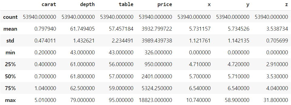
스크린샷을 보면 알 수 있는데, numeric이 아닌 cur, color, clarity 등은 describe()에 나타나지 않는 것을 알 수 있다.
dataframe 전체에 mean(), std() 등을 계산할 수 있다. 이때 head(), tail()과 같이 계산할 범위를 지정할 수도 있다.
df.mean()

<ipython-input-15-c61f0c8f89b5>:1: FutureWarning: Dropping of nuisance columns in DataFrame reductions (with 'numeric_only=None') is deprecated; in a future version this will raise TypeError.  Select only valid columns before calling the reduction.
  df.mean()
carat       0.797940
depth      61.749405
table      57.457184
price    3932.799722
x           5.731157
y           5.734526
z           3.538734
dtype: float64


df.head(50).mean()
<ipython-input-16-56442511a41d>:1: FutureWarning: Dropping of nuisance columns in DataFrame reductions (with 'numeric_only=None') is deprecated; in a future version this will raise TypeError.  Select only valid columns before calling the reduction.
  df.head(50).mean()
carat      0.2666
depth     61.6340
table     57.8000
price    367.6800
x          4.1272
y          4.1506
z          2.5506
dtype: float64
(2023.10.24 추가) ※ Warning 에 대하여:
df.mean() 과 같은 경우 모든 column이 numeric attribute가 아닐 수 있다.
우리가 원하는 컬럼(그리고 numeric이 확실한)에 대하여 직접 mean() 등을 하는 것이 권장된다.
e.g. df['carat'].mean(), df['price'].std()
Data sclicing
컬럼 데이터를 추출할 때는 [ ] 안에 컬럼명을 문자열로 입력한다. (python dictionary와 비슷한 인덱싱)
컬럼명이 '공백이 없는 문자열'이라면 . 를 이용하여 직접 컬럼 데이터를 지정할 수 있다.
df['carat'].head()
# carat은 공백이 없는 문자열이므로
# df.carat.head() 역시 동일한 결과를 얻는다.

0    0.23
1    0.21
2    0.23
3    0.29
4    0.31
Name: carat, dtype: float64
컬럼 데이터 역시 mean(), std(), describe() 등을 통해 기본 통계량을 계산할 수 있다.
df['price'].mean()  # 3932.799721913237

df['price'].describe()
count    53940.000000
mean      3932.799722
std       3989.439738
min        326.000000
25%        950.000000
50%       2401.000000
75%       5324.250000
max      18823.000000
Name: price, dtype: float64
Groupby
diamonds dataset의 cut은, 다이아몬드의 품질을 나타내므로, 이를 이용하여 grouping을 해보자.
df_cut = df.groupby('cut')
df_cut

<pandas.core.groupby.generic.DataFrameGroupBy object at 0x7fe5a9320820>
groupby 자체로는 주피터노트북(코랩 노트북 등)에서는 주소값만 출력한다.
groupby를 하고 aggregate 함수를 이용하면 그 결과의 type이 dataframe이다.
print(type(df_cut))
<class 'pandas.core.groupby.generic.DataFrameGroupBy'>

print(type(df_cut.mean()))
<class 'pandas.core.frame.DataFrame'>
df_cut = df.groupby('cut')
df_cut.mean()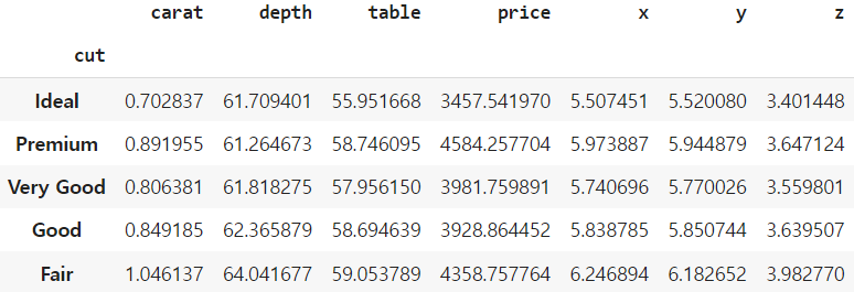
groupby를 하고, 특정 컬럼의 결과만 보고싶을 때, aggregate 이후는 dataframe이므로 똑같이 인덱싱을 하면된다.
df.groupby('cut')['price'].median()
# type: pandas.core.series.Series

cut
Ideal        1810.0
Premium      3185.0
Very Good    2648.0
Good         3050.5
Fair         3282.0
Name: price, dtype: float64
컬럼을 여러개 지정할 수 있다.
df.groupby('cut')['price', 'depth'].median() # deprecated, use list

df.groupby('cut')[['price', 'depth']].median()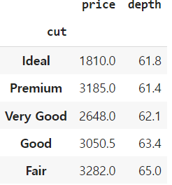
위에서 list를 이용하지 않으면 deprecated라면서 warning이 출력된다.
groupby 후 aggregate의 결과를 dataframe으로 보고 싶으면 (컬럼 개수와 상관없이) 리스트의 형태로 인덱싱을 하면 된다.
df.groupby('cut')[['carat']].median()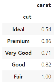
groupby의 key는 multiple column이 가능하다.
df.groupby(['cut', 'clarity'])[['price']].mean()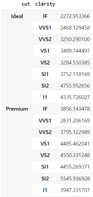
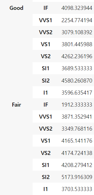
pandas의 groupby는 기본적으로 sort=True이다.
groupby의 성능을 높이고 싶다면 (대신 가독성은 떨어질 것이다) sort=False로 하면 된다.
Filtering
depth가 65 초과인 record를 필터링해보자. bool 연산을 이용하여 True/False로 making이 되고, 이중 True인 record만 필터링되는 과정을 거친다.
df_selected = df[ df['depth'] > 65 ]
df_selected.head()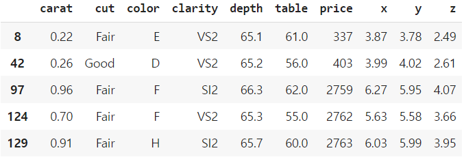
df_premium = df[df['cut'] == 'Premium']
df_premium.head()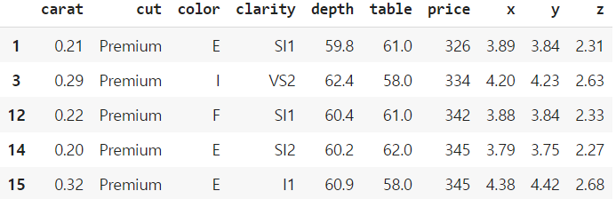
당연히, groupby와 동시에 사용할 수 있다. NaN이 출력되는 이유는, 필터링을 하면서 (depth > 65) 해당하는 record가 없기 때문이다.
df[df['depth'] > 65].groupby('cut')['price'].mean()

cut
Ideal        10791.200000
Premium               NaN
Very Good             NaN
Good          3997.842105
Fair          4334.027167
Name: price, dtype: float64
loc와 iloc를 이용한 slicing
loc는 label based로 동작한다. (boolean 허용). 따라서 [start, end]로 동작한다.
iloc는 integer position based로 동작한다(boolean 허용). 따라서 [start, end)로 동작한다.
df.loc[50:55, ['depth', 'price', 'x']]
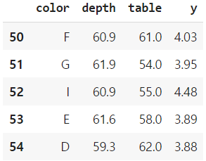
df.iloc[50:55, [2, 4, 5, 8]]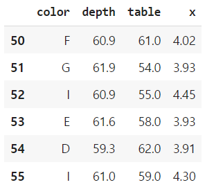
Sorting the Data
table을 기준으로 정렬해보자.
기본 정렬은 오름차순이다.
df_sorted = df.sort_values(by='table')
df_sorted.head()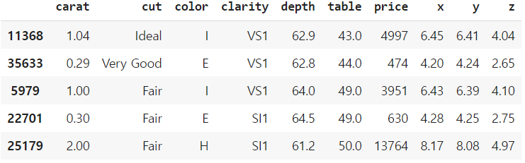
내림차순으로 바꾸고 싶으면, ascending=False를 해준다.
df_sorted = df.sort_values(by='table', ascending=False)
df_sorted.head()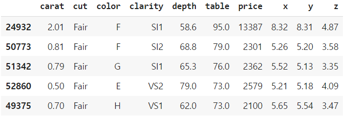
inplace=True를 사용하면, (새로운 변수에 할당하지 않고) 원래 dataframe에 적용된다.
다시 원래대로 되돌리고 싶다면, index는 변하지 않았으므로 sort_index()를 이용한다.
df.sort_values(by='price', ascending=False, inplace=True)
df.head()

df.sort_index(axis=0, ascending=True, inplace=True)
df.head()
정렬 기준이 되는 key 역시 2개 이상이 가능하다.
price는 내림차순으로, depth는 오름차순으로 정렬해보자.
df_sorted = df.sort_values(by=['price', 'depth'], ascending=[False, True])
df_sorted.head()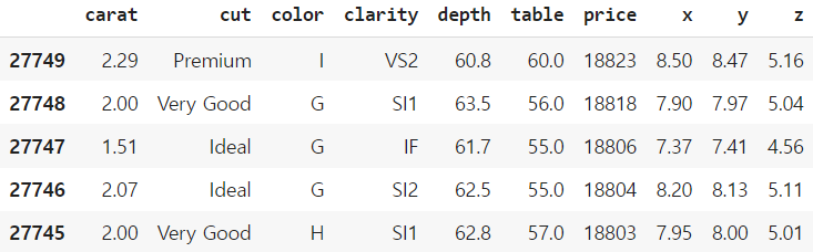
Missing Values
df = sns.load_dataset('titanic')
df[df.isnull().any(axis=1)].head()
isnull() 또는 isna()를 이용하여 결측치를 찾을 수 있다.
원래 R에서는 null과 na를 구분했지만, python에서는 구별하지 않는다.
python의 pandas는 numpy로도 기반이 있기 때문에 nan 역시 구별하지 않는다.
df.isnull().sum() # df.isna().sum()

survived         0
pclass           0
sex              0
age            177
sibsp            0
parch            0
fare             0
embarked         2
class            0
who              0
adult_male       0
deck           688
embark_town      2
alive            0
alone            0
dtype: int64
결측치를 해결하는 방법은 통계적인 여러 방법이 있지만, 여기서는 간단히 없애는 방법과 하나의 값으로 채우는 방법을 알아보자.
dropna()를 이용하여 하나라도 null인 data를 삭제하는 방법
fillna()를 이용하여 결측치를 지정한 값으로 채우는 방법
이렇게 두가지 방법이 있다.
df_drop = df.dropna()
df_drop.isna().sum() # 0

df_fill = df['age'].fillna(20)
print(df_fill.isnull().any())
df_fill

False
0      22.0
1      38.0
2      26.0
3      35.0
4      35.0
       ...
886    27.0
887    19.0
888    20.0
889    26.0
890    32.0
Name: age, Length: 891, dtype: float64
Aggregation
다시 다이아몬드 데이터로 돌아와서 agg를 이용해보자
df[['table', 'price']].agg(['min', 'max', 'mean', 'median'])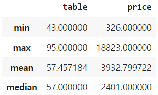
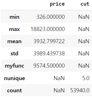
컬럼마다 다른 agg 함수를 적용할 수 있다.
심지어 user-defined 함수를 이용할 수도 있다.
def myfunc(x):
    x = sorted(x)
    return (x[0] + x[-1])/2

df.agg({
    'price': [min, max, 'mean', 'std', myfunc],
    'cut': ['nunique', 'count']
})
'스터디 > 데이터사이언스' 카테고리의 다른 글
| [Python] 선형회귀 모델링 (0) | 2023.04.12 |
|---|---|
| [Python] 데이터 시각화 (Basic) (0) | 2023.04.11 |
| [Data Science] Grubb's test를 이용한 Outlier detection (0) | 2023.04.08 |
| [Data Science] Association Rule Mining (7) mlxtend로 association rule을 만들어보자 (0) | 2023.04.04 |
| [Data Science] Association Rule Mining (6) Interesting Measures (0) | 2023.04.03 |


