728x90
반응형
Setup
bagging과 random forest를 실습하기 위해 필요한 라이브러리를 import하자.
# To support both python 2 and python 3
from __future__ import division, print_function, unicode_literals

# Common imports
import numpy as np
import os

# to make this notebook's output stable across runs
np.random.seed(42)

# To plot pretty figures
%matplotlib inline
import matplotlib as mpl
import matplotlib.pyplot as plt
from matplotlib.colors import ListedColormap

mpl.rc('axes', labelsize=14)
mpl.rc('xtick', labelsize=12)
mpl.rc('ytick', labelsize=12)

# dataset
from sklearn.model_selection import train_test_split
from sklearn.datasets import make_moons

# Ensemble model and Decision-tree
from sklearn.ensemble import BaggingClassifier
from sklearn.tree import DecisionTreeClassifier

# metric
from sklearn.metrics import accuracy_score
사용할 데이터셋은 make_moon을 이용한 2개의 초승달 모양의 2차원 데이터이다.
X, y = make_moons(n_samples=500, noise=0.30, random_state=42)
X_train, X_test, y_train, y_test = train_test_split(X, y, random_state=42)
moon data를 시각화하기 위한 함수이다.
def plot_decision_boundary(clf, X, y, axes=[-1.5, 2.5, -1, 1.5], alpha=0.5, contour=True):
    x1s = np.linspace(axes[0], axes[1], 100)
    x2s = np.linspace(axes[2], axes[3], 100)
    x1, x2 = np.meshgrid(x1s, x2s)
    X_new = np.c_[x1.ravel(), x2.ravel()]
    y_pred = clf.predict(X_new).reshape(x1.shape)
    custom_cmap = ListedColormap(['#fafab0','#9898ff','#a0faa0'])
    plt.contourf(x1, x2, y_pred, alpha=0.3, cmap=custom_cmap)
    if contour:
        custom_cmap2 = ListedColormap(['#7d7d58','#4c4c7f','#507d50'])
        plt.contour(x1, x2, y_pred, cmap=custom_cmap2, alpha=0.8)
    plt.plot(X[:, 0][y==0], X[:, 1][y==0], "yo", alpha=alpha)
    plt.plot(X[:, 0][y==1], X[:, 1][y==1], "bs", alpha=alpha)
    plt.axis(axes)
    plt.xlabel(r"$x_1$", fontsize=18)
    plt.ylabel(r"$x_2$", fontsize=18, rotation=0)
Bagging
# define BaggingClassifier
bag_clf = BaggingClassifier(
    DecisionTreeClassifier(random_state=42), n_estimators=500,
    max_samples=100, bootstrap=True, n_jobs=-1, random_state=42
)

# fitting the training data
bag_clf.fit(X_train, y_train)

# predict
y_pred = bag_clf.predict(X_test)

# accuracy
print(accuracy_score(y_test, y_pred)) # 0.904

# compare with Single DecisionTreeClassifier
tree_clf = DecisionTreeClassifier(random_state=42)
tree_clf.fit(X_train, y_train)
y_pred_tree = tree_clf.predict(X_test)
print(accuracy_score(y_test, y_pred_tree)) # 0.856- n_estimators=500: 500개의 DecisionTreeClassifier를 앙상블할 것이다.
- max_samples=100: X(fit 할때 넘겨주는 X_train) 에서 추출할 sample 수
- bootstrap=True: sampling 방법은 bootstrap sampling을 이용한다.
- n_jobs=-1: 가능한 모든 CPU 자원을 사용한다.
- random_state=42: 재현성을 위해 랜덤 시드를 42로 한다.
반응형
# figure size setting
plt.figure(figsize=(11,4))

# plot single decision tree classifier
plt.subplot(121)
plot_decision_boundary(tree_clf, X, y)
plt.title("Decision Tree", fontsize=14)

# plot ensemble model (500 decision tree classifier)
plt.subplot(122)
plot_decision_boundary(bag_clf, X, y)
plt.title("Decision Trees with Bagging", fontsize=14)

# plot all
plt.show()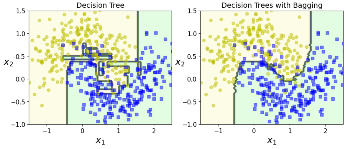
Out-of-Bag Evaluation (OOB Score)
OOB score를 보고 싶다면 bagging classifier를 fitting할 때 해당 옵션을 설정해야한다.
# oob score
bag_clf_2 = BaggingClassifier(
    DecisionTreeClassifier(splitter="random", max_leaf_nodes=16, random_state=42),
    n_estimators=500, max_samples=1.0, bootstrap=True, n_jobs=-1, random_state=42,
    oob_score=True
)
bag_clf_2.fit(X_train, y_train)

print(bag_clf_2.oob_score_) # 0.92

y_pred_2 = bag_clf_2.predict(X_test)
print(accuracy_score(y_test, y_pred_2)) # 0.92
oob evaluation의 결과가 0.92를 얻었다. 이는 test set에서 약 92%의 정확도를 갖는 성능을 갖는다.
실제 y_test와 y_pred_2의 accuracy를 비교하면 0.92이다.
(데이터셋이 간단해서 동일하게 나왔다. 실제로는 약간 차이가 있을 수 있다. 그러나 여전히 oob_score와 실제 testset의 결과는 비슷할 것이다.)
Random Forests
동일한 moon dataset에 대하여 random forest를 학습시켜보자.
from sklearn.ensemble import RandomForestClassifier

rnd_clf = RandomForestClassifier(n_estimators=500, max_leaf_nodes=16, n_jobs=-1, random_state=42)
rnd_clf.fit(X_train, y_train)

y_pred_rf = rnd_clf.predict(X_test)

# almost identical predictions
np.sum(y_pred == y_pred_rf) / len(y_pred) # 0.976- n_estimators=500: 500개의 decision tree를 학습하여 앙상블
- max_leaf_nodes=16: 각 tree는 최대 16개의 leaf node를 갖도록 제한
- n_jobs=-1 (생략)
- random_state=42: (생략)
Feature Importance (Variable Importance)
iris dataset에서도 적용해보자.
사이킷런 random forest는 자체적으로 feature importance를 계산한다. (이들의 합은 $1$이다)
from sklearn.datasets import load_iris
iris = load_iris()

# train the Random-Forest-Classifier
rnd_clf = RandomForestClassifier(n_estimators=500, n_jobs=-1, random_state=42)
rnd_clf.fit(iris["data"], iris["target"])

# print feature importances
for name, score in zip(iris["feature_names"], rnd_clf.feature_importances_):
    print(name, score)

'''
sepal length (cm) 0.11249225099876375
sepal width (cm) 0.02311928828251033
petal length (cm) 0.4410304643639577
petal width (cm) 0.4233579963547682
'''

print(rnd_clf.feature_importances_)
# array([0.11249225, 0.02311929, 0.44103046, 0.423358  ])
2D data (pixel importance)
# load MNIST dataset
try:
    from sklearn.datasets import fetch_openml
    mnist = fetch_openml('mnist_784', version=1)
    mnist.target = mnist.target.astype(np.int64)
except ImportError:
    from sklearn.datasets import fetch_mldata
    mnist = fetch_mldata('MNIST original')

# define and fit the RandomForestClassifier
rnd_clf = RandomForestClassifier(n_estimators=10, random_state=42)
rnd_clf.fit(mnist["data"], mnist["target"])

# function to display the feature importance of classifier
def plot_digit(data):
    image = data.reshape(28, 28)
    plt.imshow(image, cmap = mpl.cm.hot,
               interpolation="nearest")
    plt.axis("off")

# display the feature importances of digit
plot_digit(rnd_clf.feature_importances_)

cbar = plt.colorbar(ticks=[rnd_clf.feature_importances_.min(), rnd_clf.feature_importances_.max()])
cbar.ax.set_yticklabels(['Not important', 'Very important'])

plt.show()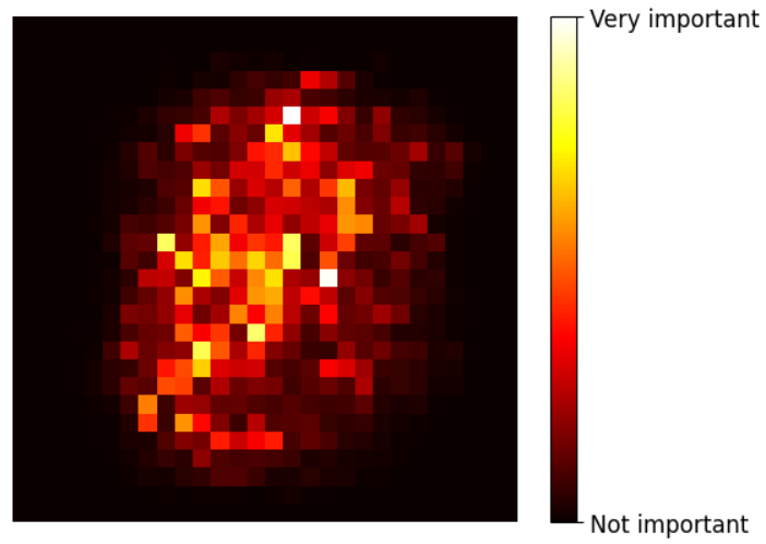
Random Forest는 어떤 feature가 중요한지 매우 쉽게 파악할 수 있다. (이를 이용하여 feature selection에도 활용할 수 있다)
728x90
반응형
'스터디 > 인공지능, 딥러닝, 머신러닝' 카테고리의 다른 글
| [Ensemble] AdaBoost in Python (scikit-learn) (0) | 2023.05.16 |
|---|---|
| [Ensemble] AdaBoost (0) | 2023.05.16 |
| [Ensemble] Random Forests (0) | 2023.05.12 |
| [Ensemble] Basic Concept of Ensemble Methods, Bagging, Boosting (0) | 2023.05.12 |
| [Machine Learning] SVM in Python (2) - Margin, Regularization, Non-linear SVM, Kernel (0) | 2023.05.11 |


